Binary Logistic Regression
In some situations, Lean Six Sigma practitioners find a Y that is discrete and Xs that are continuous. How can we apply regression in these cases? Black Belt training indicated that the correct technique is something called b inary logistic regression or binary regression. But this tool is often not well understood.

An example about a well-known space shuttle accident can help to demystify logistic regression using the simplest logistic regression – binary logistic regression (binary regression), where the Y has just two potential outcomes (i.e., “yes” or “no”).
The data in Table 1 comes from the Presidential Commission on the Space Shuttle Challenger Accident (1986). The data consists of the number of the flight, the air temperature in Fahrenheit at the time of the launch and whether or not there was damage to the booster rocket field joints. Using binary logistic regression and given a particular temperature at launch time, this data can help to determine the probability of damage to the booster rocket field joints.
There are five steps to apply logistics regression.

Step 1. Plot the Data
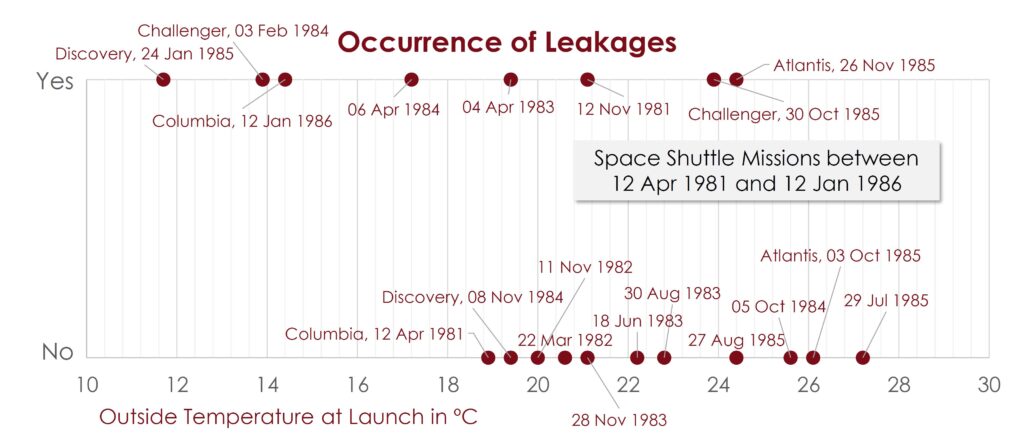
A stratified dot plot might help to graphically display the data for binary regression. It is obvious from Figure 1 that the probability of damage is greater at lower temperatures.

However, there is quite a fair bit of overlap in the distribution. Is launch temperature a real X (i.e., a real predictor of damage)? And if so, what is the probability of damage for any given launch temperature?
Step 2. Formulate the Binary Logistic Regression Model
Any regression requires a continuous output or Y. However, in this case the Y is discrete with only two categories or two events: Damage – yes or no. What to do? The “trick” behind the logistic regression is to turn the discrete output into a continuous output by calculating the probability (p) for the occurrence of a specific event. That means, the logistic regression provides a model to predict the p for a specific event for Y (here, the damage of booster rocket field joints, p = P[Y=1]) given any value of X (here, the temperature at the time of the launch). The logistic regression equation has the form:
ln(p/(1-p) = β0 + β1 X
This function is the so-called “logit” function where this regression has its name from. The procedure for modeling a logistic model is determining the actual percentages for an event as a function of the X and finding the best constant and coefficients fitting the different percentages.
This is exactly the equation that comes out of statistical software’s output for logistics regression:
ln(p / (1-p) = 14.204 – 0.226 Temperature
Step 3. Check the Validity of the Regression Model
There are two major checks that test the validity of this model:
- P-value for the coefficient is less than 0.05.
A p-value is calculated for each coefficient. If the p-value is low then there is a significant relationship between the X variable and the Y. In this case, the coefficient for temperature has a p-value of 0.042 (i.e., there is a significant relationship between the temperature and the probability of a damage). - P-value of the “goodness of fit” tests are greater than 0.05.
Goodness-of-fit tests are conducted to see whether the model adequately fits the actual situation. Low p-values indicate a significant difference of the model from the observed data. Hence, the p-values should be above 0.05 to show that there are no significant differences between the predicted probabilities (from the model) and the observed probabilities (from the raw data). In this case, from the goodness-of-fit tests, none of them show a significant difference – the regression model is valid.
Step 4. Reverse the Logit Equation
Reversing the Logit equation helps to obtain an answer to the question, given a particular setting of X, what is the probability of failure? Reversing this, the result is:
p = (e exp(14.204 – 0.226 Temperature)) / ((1+e exp(14.204 – 0.226 Temperature)))
with e = 2.71828.
On the day of the Challenger incident, the temperature was 31 degree Fahrenheit (-0.6 degree Celsius). Hence, the probability of damage to the booster rocket field joints on that day is:
p = (e exp(14.204 – 0.226 x 31)) / ((1+e exp(14.204 – 0.226 x 31))) = 0.999
Hence, damage was almost a certainty.
Step 5. Visualize the Results (Optional)
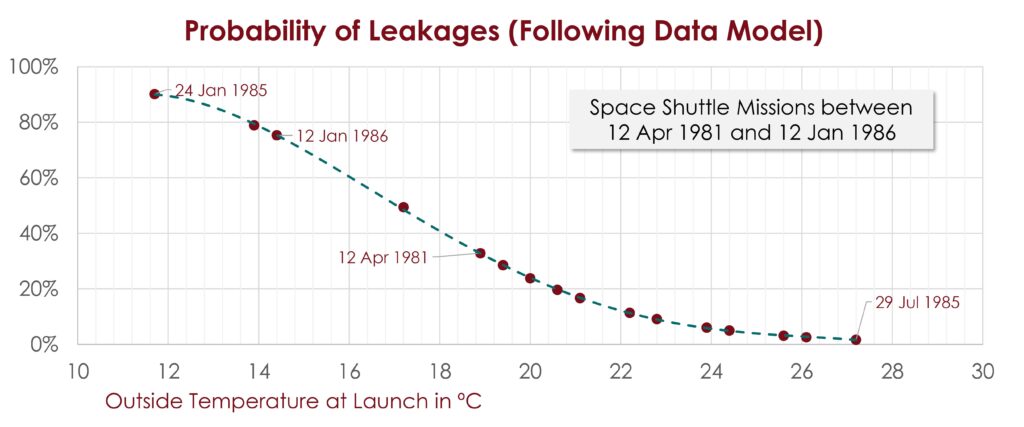
The event probability for all the possible temperature settings is the result of applying the binary regression model. Using this event probability, we produce the scatter plot (decreasing logistic plot) in Figure 2.

Using this scatter plot, it is quite easy to do some prediction. For example, if the outside temperature is about 55 degree F (12.6 degree Celsius), the probability of getting a damage – or better a leak in the booster rocket – is more than 85%.

