Making Sense of Test for Equal Variances
Three teams compete in our CHL Business Simulation, CHL Red, CHL Green and CHL Blue.
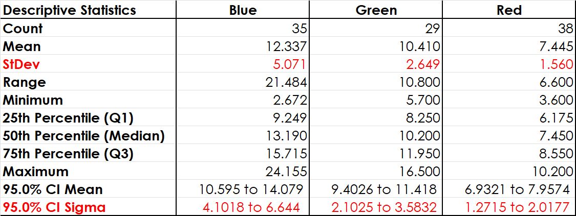
After completing Day One, it looks like the teams show a very different performance. Although the means look very similar, the variation is strikingly different. This is surprising, since all teams start with exactly the same prerequisites. To test this assumption of different variability among the teams, the Test for Equal Variances is deployed.
Finding a significant difference in variances (square of standard deviation), in the variation of different data sets is important. These data sets could stem from different teams performing the same job. If they show a different variation, it usually means, that different procedures are used to perform the same job. Looking into this may offer opportunities for improvement bu learning from the best. However, this only makes sense if this difference is proven, i.e. statistically significant.
To perform the Test for Equal Variances, we take the following steps:
1. Plot the Data
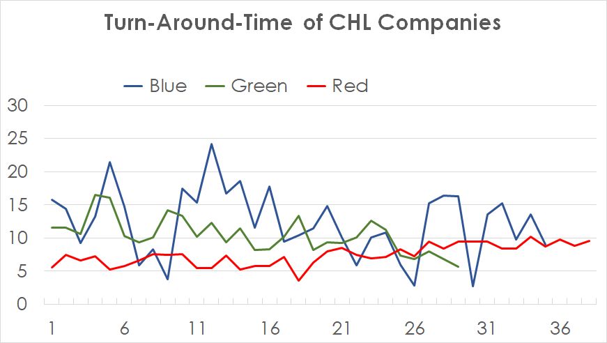
For any statistical application, it is essential to combine it with a graphical representation of the data. Several tools are available for this purpose. They include the popular stratified histogram, dotplot or boxplot. The Time Series Plot at Figure 1 does not clearly show the variability of the three teams.
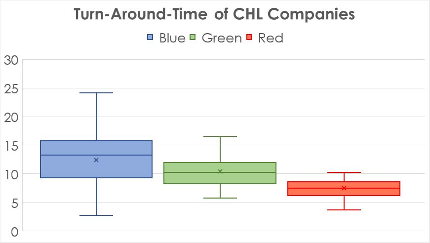
The boxplot in Figure 2 shows much better an obvious difference in the variation between the three groups. A statistical test can help to calculate the risk for this decision.
2. Formulate the Hypothesis for Test For Equal Variances
In this case, the parameter of interest is an average, i.e. the null-hypothesis is
H0: σBlue = σGreen = σRed,
with all σ being the population standard deviation of the three different teams.
This means, the alternative hypothesis is
HA: At least one σ is different to at least one other σ.
3. Decide on the Acceptable Risk
Since there is no reason for changing the commonly used acceptable risk of 5%, i.e. 0.05, we use this risk as our threshold for making our decision.
4. Select the Right Tool
If there is a need for comparing variances, there are at least three popular tests available:
- For two normally distributed data sets: F-test,
- For more than two normally distributed data sets: Bartlett’s test and
- For two or more non-normally distributed data sets: Levene’s test.
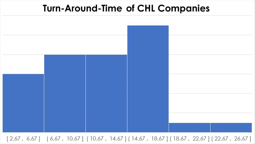
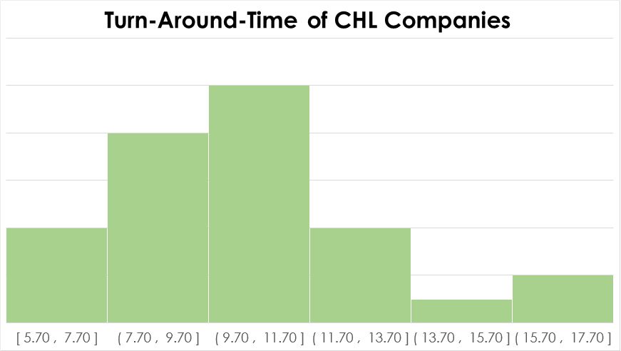
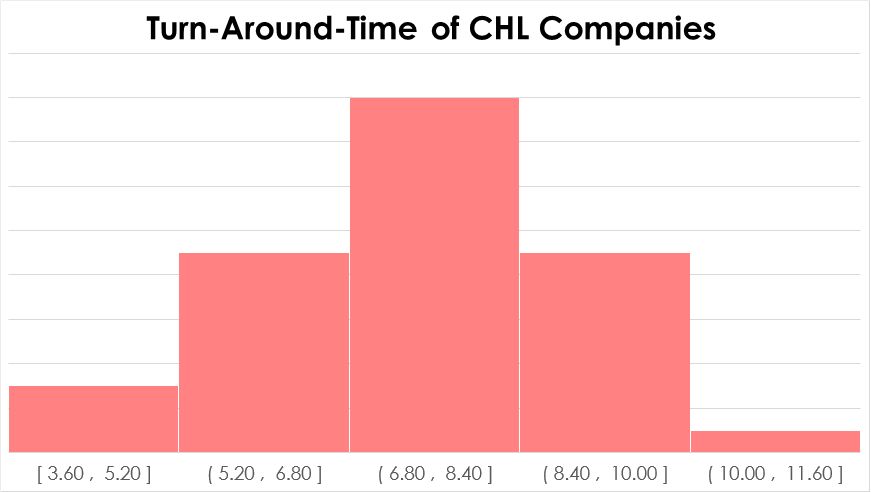
Since tests that are based on a certain distribution are usually sharper, we need to check whether we have normal data. Figure three reveals, that CHL Blue does not show normality following the p-value of the Anderson-Darling Normality Test. Therefore, we need to run a Test for Equal Variances following Levene’s test.
5. Test the Assumptions
Finally, there are no other prerequisites for running a Levene’s test.
6. Conduct the Test
Running the test delivers a p-value of 0.0000, i.e., there is no doubt whatsoever that the variation between the CHL groups is different.
The following table shows the pairwise comparison p-values. This explains that all variances are different from each other.

7. Make a Decision
With this, the Levene’s statistics means that there is at least one significant difference.
Additionally, this statistics shows which CHL is different from which other CHL. The p-value for Levene Pairwise Probabilities is 0.0000 between CHL Blue and CHL Green, as well as between CHL Green and CHL Red, i.e. there is a significant difference between CHL Blue and CHL Green as well as between CHL Green and CHL Red. The boxplot shows the direction of this difference.
Finally, the statistics informs that CHL Red seems to have a significantly better way to run the simulation with much less variation, i.e. StDev of 1.56min compared to 2.65 and 5.07, respectively. After further looking into the procedure, we recognise that CHL Green organises packages in First-in-First-out (FIFO) order, whereas CHL Blue and CHL Red do not always ensure FIFO.
Interested in the stats? Read here.


