Consider a production process that produced 10,000 widgets in January and experienced a total of 112 rejected widgets after a quality control inspection (i.e., failure rate = 1.12%). A Six Sigma project was deployed to fix this problem and by March the improvement plan was in place. In April, the process produced 8,000 widgets and experienced a total of 63 rejects (failure rate = 0.79%). Did the process indeed improve?
The appropriate hypothesis test for this question is the two-proportions test.
As the name suggests it is used when comparing the percentages of two groups. It only works, however, when the raw data behind the percentages (100 rejects out of 10,000 parts produced and 63 out of 8,000 respectively) is available since the sample size is a determining factor for the test statistics.
To perform this test, we take the following steps:
1. Plot the Data
For any statistical application, it is essential to combine it with a graphical representation of the data. The selection of tools for this purpose is limited. They include pie chart, column chart and bar chart.
The pie chart in Figure 1 shows that the percentage of defective widgets has gone down from January to April. However, there is not a large drop. Therefore, based on this plot, it is risky to draw a conclusion that there is a significant (i.e. statistically proven) difference between the defect rate in January and that in April. A statistical test can help to calculate the risk for this decision.
2. Formulate the Hypothesis for Two-Proportions Test
In this case, the parameter of interest is a proportion, i.e. the null-hypothesis is
H0: PJanuary = PApril,
with PJanuary and PApril being the real defect percentage for these two months.
This means, the alternative hypothesis is
HA: PJanuary ≠ PApril.
3. Decide on the Acceptable Risk
Since there is no reason for changing the commonly used acceptable risk of 5%, i.e. 0.05, we use this risk as our threshold for making our decision.
4. Select the Right Tool
If there is a need for comparing two proportions, the popular test for this situation is the two-proportions test.
5. Test the Assumptions
There are no prerequisites for the application of this test.
6. Conduct the Test
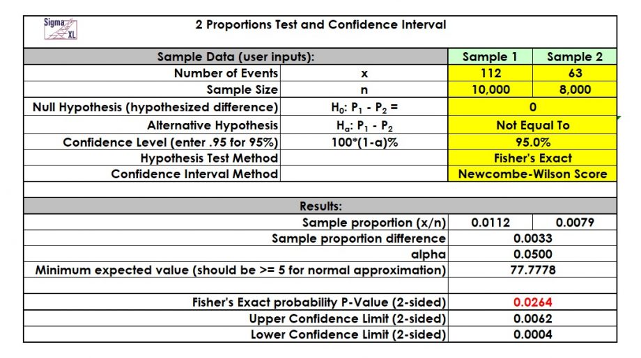
Using the two-proportions test, statistics software SigmaXL generates the output in Figure 2.
Since the p-value is 0.0264, i.e. less than 0.05 (or 5 percent), we reject H0 and accept HA.
7. Make a Decision
As a result, rejecting H0 means that there is evidence for a significant difference between the January and the April batch. The risk for being wrong with this assumption is only 2.64%.
In conclusion, we can trust the change in the widget production line and expect improved quality under the new conditions.
Interested in the stats? Read here.


