- +65 61000 263
- Contact@COE-Partners.com
- Newsletter
Lean Six Sigma MEASURE Phase
Lean Six Sigma MEASURE Phase
In the Lean Six Sigma DEFINE phase, a high-level process map has been developed and the voice of the customer has been collected. In the Lean Six Sigma MEASURE phase, potential root causes for the problem will be determined, data for problem and potential root causes will be collected and the actual process performance will be established. This data will be used in ANALYSE to distinguish between vital few and trivial many root causes – the most important prerequisite for IMPROVE.
The principal task of Lean Six Sigma MEASURE phase is the data collection.
The following list of tasks may not be needed for all Lean Six Sigma projects, on the one hand. On the other hand, some projects may even require additional tasks to be completed. The list of tasks required depends on the problem that needs to be solved and the data that needs to be handled.
1. Identify Potential Root Causes
Data for outcome variables (Y) and potential causes (Xs) are normally collected at the same time under the same conditions. In addition, data on stratifying factors, such as time, persons, layer, place and product type, are recorded. The goal of this step is to identify potential causes that should be included in the data collection.
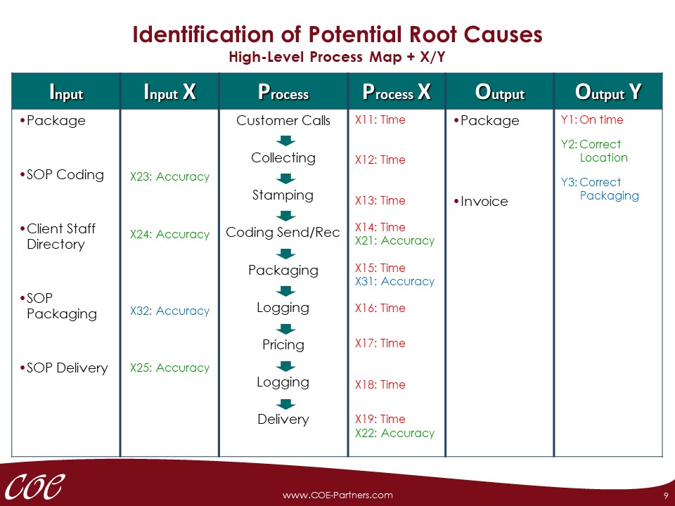
While the outcome variable (Y) or variables (Ys) were determined in the step of understanding the voice of the customer (VOC), variables are to be found as potential causes in the process inputs and process steps. The discovery of these input and process variables is therefore based on the SIPOC or high-level value stream map (VSM) and on the knowledge and experience of the process participants, who are responsible for the process on a daily basis.
Causes for the problem may be due to certain parameters of the process or of the inputs. Since the generation of these parameters cannot usually be automated, the result depends on the completeness of the SIPOC or VSM as well as the presence of employees who are familiar with the process. Process step for process step, the question is posed as to whether the respective step can affect the result, i.e. whether the corresponding step can be the cause of the problem.
In principle, two main categories of parameters can be used. The first category deals with the time required for certain steps. This category is important when the problem is time-relevant such as “late delivery” or turn-around-time. The second category includes errors in process steps or inputs, which always play a greater role when the problem manifests itself in errors such as “wrong location”. Both categories are strongly linked. For instance, errors in process steps can lead to internal post-processing and thus to longer turn-around-time.
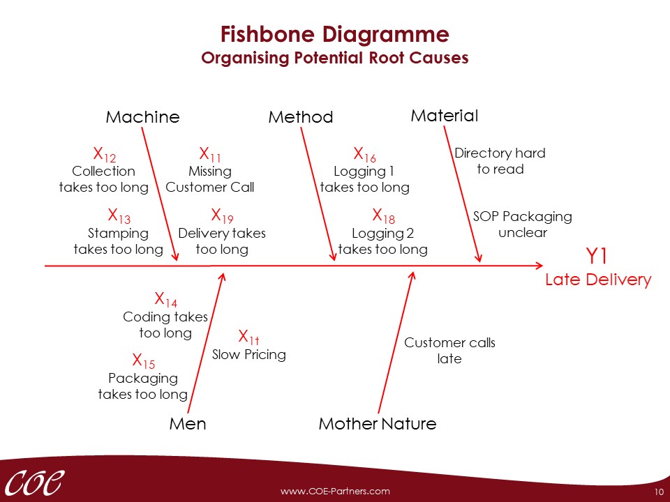
The result of Task 1 is a list of potential causes of error (Xs), which should be classified into categories in order to get an overview on the one hand, and to check completeness on the other. Both standard categories such as Machine, Method, Material, Men (human) and Mother Nature or project-specific categories can be used. The standard categories have proven to be advantageous when checking for completeness.
For this purpose, a fish bone diagram is recorded on a sufficiently large writing surface formed by a wall, a white board or several flipchart sheets combined. In the head of the fish, the problem named in the project charter is displayed. A process output variable (Y, CTQ) should be used. Business cases such as the loss of customers or customer-related measures such as customer satisfaction should not be shown in the head of the fish.
At the main bones the headings for the categories are formed. Subsequently, the collected potential causes are assigned to the corresponding categories or bones. The potential causes have, of course, overlapping, that is, multiple references. In addition, there are associated causes, that is, an X can be a sub-point for another X. This does not pose an issue as long as the potential cause becomes part of main bones or sub bones or branches.
After creating the fish bone diagram with potential root causes (Xs) for problem (Y), select the Xs for which data is to be collected. This selection can be made using the existing fish bone diagram or by means of a prioritisation matrix.
A somewhat less elaborate method for selecting candidate Xs for data collection is the use of multi-voting at the fish bone diagram. For each X in the diagram, the following is asked:
- Is there theoretically a weak, moderate, or strong relationship between X and Y, that is, X can exert an influence on Y?
- Does this influence actually occur, that is, the cause, “Directory hard to read” has already been observed in the past?
The answers are used to determine whether the data collection for this X makes sense or not. In case of disagreements, the team members should be very precise in explaining their position. If there is no clear “no”, the X cannot be deleted from the data collection.
In addition to potential problems, it is useful to detect the conditions as stratifying factors for the occurrence of the problem. The conditions are not a problem but can help in the analysis of causes. These factors are typically recorded with the questions of who, when, where, what, how. For example, it is important to know which customer has sent a package. There could be a systematic difference in the processing time for different locations. Or, there could be a time-dependent difference, i.e. packages sent early take a different time than later packages. The underlying factor could be a function of fatigue.
These stratifying factors must be assignable to the data acquired during the data collection. It is therefore necessary to include these variables in the data collection.
This step has the following deliverables:
- A fishbone diagram with clusters of potential root causes like machine, method, material, man and mother nature or project specific clusters that have become apparent during development of potential root causes,
- A list of potential root causes that have been selected for data collection based on process knowledge and experience of team members.
2. Analyse Measurement System
Before data for outcome variable (Y) and potential causes (Xs) are collected, the corresponding measurement systems have to be analysed. Measurement systems may cause various errors that can make the analysis of the process variation more difficult or impossible.
The goal of this step is therefore to analyse the variation resulting from measurement systems and to eliminate or to minimise it in order to ensure the usefulness of the data to be collected. The methods for measurement system analysis are tailored to the respective data types – continuous data and attribute data. Continuous data are quantitative, measurable, variable data, for instance, dimensions, time, weight. Attribute data are qualitative, discrete, countable data as number of errors, number of features. Attribute data with large frequency may be treated as continuous data.
Measurement systems must ensure accuracy, repeatability, reproducibility and stability of the measurement results.
Accuracy means the ability of a measurement system to accurately reflect the actual value. For example, when examining a customer loan request, ignoring missing information would be an inaccuracy that could have a negative impact on the downstream process.
Repeatability is the ability of a person to be able to repeat a score for the same object under the same conditions. For example, the declining attention of someone assessing loan applications towards the end of the working day may result in an inaccuracy that would not have happened in the morning.
Reproducibility refers to the ability to conduct an assessment by different persons and/or under different conditions with exactly the same result. For example, it would be a problem for the downstream process if the outcome of a credit risk analysis were dependent on the person examining the document, which means, if the same request were accepted by one person but rejected by another.
Stability identifies the ability of the measurement system to provide the same results long-term and not to be subjected to depreciation over time.
Accuracy Correction (Calibration) and Stability Analysis are methods that are beyond the scope of this page.
The method for verifying repeatability and reproducibility is also called Gage R & R (Gauge Repeatability and Reproducibility). This Gage R & R basically uses different procedures for different data types, continuous, i.e. variable and discrete, i.e. attribute data. Both methods of analysis examine the entire system including the measurement system, the sample, the tester and the environment.
For the measurement system analysis for attribute, i.e. discrete data, better be at least 20 – 30 typical units from the process are selected in such a way that approximately half are error-free and the other half are equipped with typical errors. This selection is made by a person familiar with the quality features, the so-called master.
Then, the units are presented to persons who are normally in charge of assessing this kind of units, without letting them know the assessment result by the master. A deviation of the evaluation by the examiner compared to that of the master results in reproducibility errors.
If the repeated examination of the same units by the same examiner under the same conditions leads to a deviation, a repeatability problem exists.
Repeated testing should be performed blindly. That is, the person assessing the units must not know the result of their previous evaluation of the same unit. In practice, this is not always easy to ensure. On the other hand, similar units can be used which have the same error in order to test the repeatability of the results.
The goal for both repeatability and reproducibility is 100%. Any deviation thereof means either allowing defective units to be passed to downstream process steps or holding back proper units. If these requirements are met, data collection can start immediately. In all other cases, the measurement system must be verified for the reasons for poor repeatability or reproducibility and corrective measures must be taken.
If there are obvious differences between repeatability characteristics for different persons, training measures may be adequate to improve the quality of the measurement system for single persons. If the measurements of all persons have a repeatability problem, the measurement system, that is, the combination of method, person, measuring means, measuring device and environmental conditions, should be questioned.
In the event of a reproducibility problem, the difference between the subject and the master shall be analysed and eliminated. Causes of this problem are to be found in inadequate instruction or inadequate training for the person concerned. If many assessing persons cannot be in agreement with the master, it is necessary to check whether the requirements for a unit for achieving ‘error-free’ assessment are precisely and comprehensively specified in test instructions.
This procedure is to be repeated until the measurement system capability meets the requirements.
This step has the following deliverables:
- List of measurement systems used for data collection.
3. Plan Data Collection
The basis of a meaningful data analysis are representative data. Representative data can be collected from relatively small samples, which are gathered in a consistent manner under pre-set conditions.
The objective of this step is to determine the amount (sample size) of data needed, as well as planning the methods of data collection. The methods of calculating the sample size are different for discrete and continuous data.
The aim of data collection is usually determining either the average and the standard deviation a continuous process parameter, or determining the percentage of a discrete process parameter. Due to the nature of data collection, more often than not, sampling is the preferred method of data collection. And, it usually gives results with a certain precision.
Sample inspections can only deliver estimations to the actual process parameters. The size of the sample inspection depends on the requirements for these estimations. These requirements will be expressed with the so-called confidence interval or the precision (50% of the confidence interval). The confidence interval defines the area, where the actual value of the parameter is very likely to be found.
For example, a cycle time average of 52 minutes with a standard deviation of 8 minutes, is measured with ten measurements by a sample inspection, placing it in a confidence interval between 46.3 and 57.7 minutes, i.e. a precision of 5.7 minutes, and assuring a confidence level of 95%. This means, with a chance of 95% the real average is between 46.3 and 57.7 minutes.
As another example, finding 10 erroneous applications amongst 80 sampled applications results in an error rate of 12.5%. However, due to the sampling error, the real error percentage is to be expected between the error margins, the confidence interval, of 6.2% to 21.8% with a confidence level of 95%.
Accordingly, before data collection it is necessary to determine the size of the confidence interval for the result. It has to be taken into consideration, however, that a narrower confidence interval demands a larger sample size. But it ensures a more exact (precise) result as well.
After the desired confidence interval is established, the sample size for the data collection is to be determined. In order to estimate the sample size, it is necessary to have an approximate value for the proportion or the mean that is to be estimated. This appraisal can be achieved either through historical data, through taking into consideration the results of similar processes or through benchmarking.
If the required confidence level is set to 95%, the following formulae give a conservative estimation of the sample size to be collected:
The data collection must provide representative data, i.e. each unit of the process must get the same chance to be part of the data collection. There must not be a systematic difference between the collected data and the data which aren’t included in the sample. As an example, collecting data only in the morning would not be acceptable if the process was running the entire day.
Generally, the data collection should ensure sampled data show all of the process’s inherent variation. In the event of the sampling 100% of the data in a specific time interval, there is a high likelihood of identifying all micro-fluctuations, i.e. short-term variation, in the process. In this case, we must ensure a lack of macro-fluctuations, like seasonal differences, in the data, since these would not be detected.
The data collection plan should include the beginning and ending time of the sample collection, the designated ways of recording the results as well as the responsible personnel. For the involved individuals, a proper briefing is recommended to ensure data collection with consistent implementation.
This step has the following deliverables:
- A data collection plan showing what measurements are to be taken by whom, when, where, how, under which conditions etc.
4. Plot the Data
The most important form of data analysis is at the same time the first step, which is the graphical illustration of the collected data. There are two separable groups of graphs:
- Graphs, that give information about one variable. These graphs should be used after any data collection; therefore, they are taken into consideration in this step.
- Graphs, that show and analyse a relationship, i.e. correlation between two or more variables. These graphs will be used in the analysis phase; thus, they will be discussed in a later step.
The objective of this step is to identify patterns in data sequences, in order to set up the requirements for the ulterior data analysis.
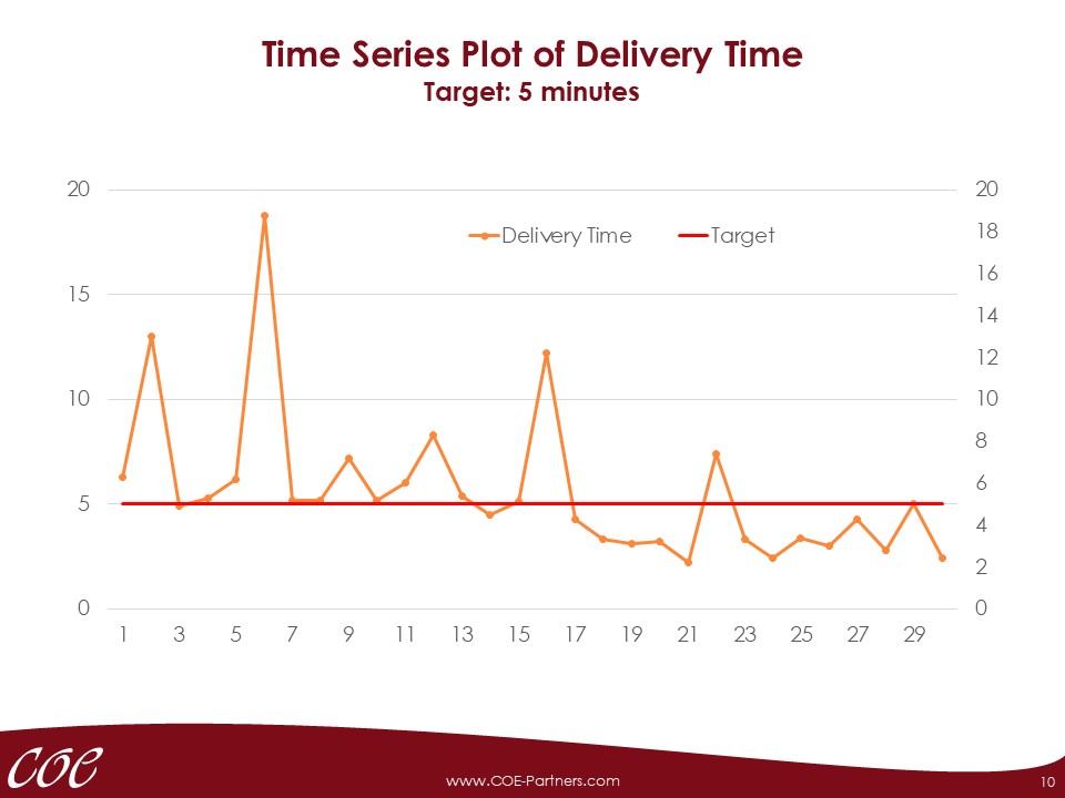
The very first task after data gathering should be a graphical illustration of the recorded data over the period of the data collection. The most important goal of such a representation is to check for potential systematic influences on the data, which are identifiable in patterns. In principle, it is desirable to have a process that shows only common cause variation, which is regarded as a stable process.
A stable process is identifiable by its nature of not showing any conspicuous patterns, instead it shows a regular spread over time.
An unstable process is recognisable by obvious patterns that are usually caused by special cause variation, driven by systematic influences.
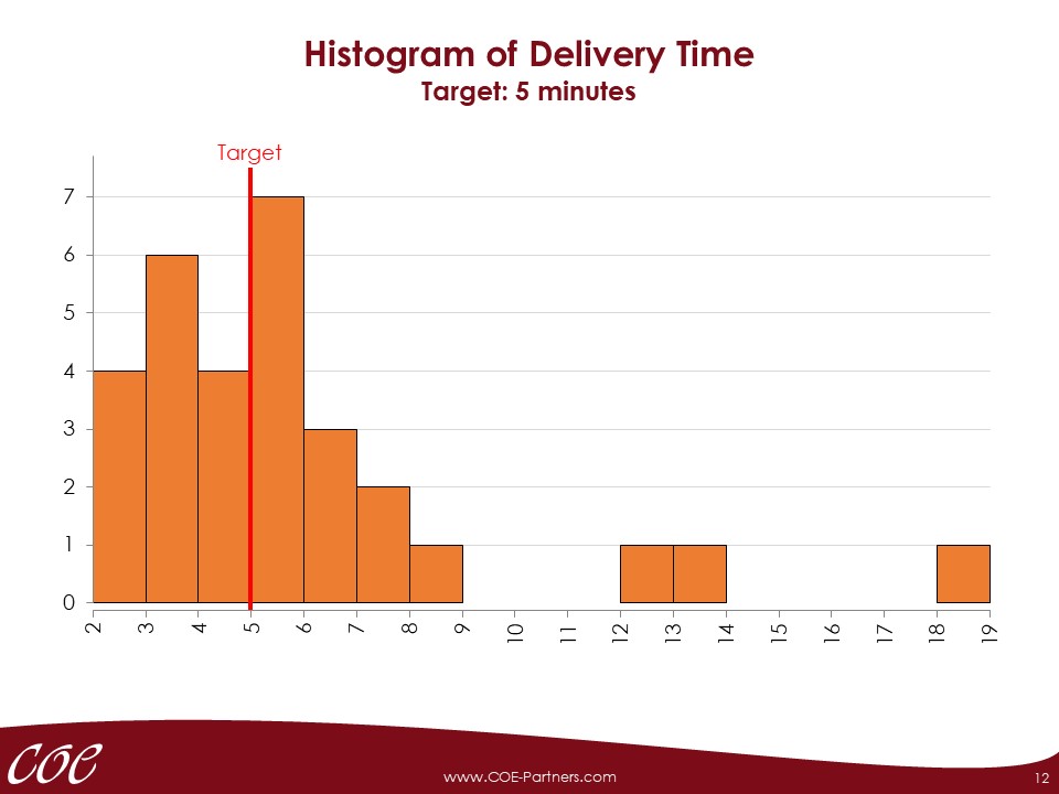
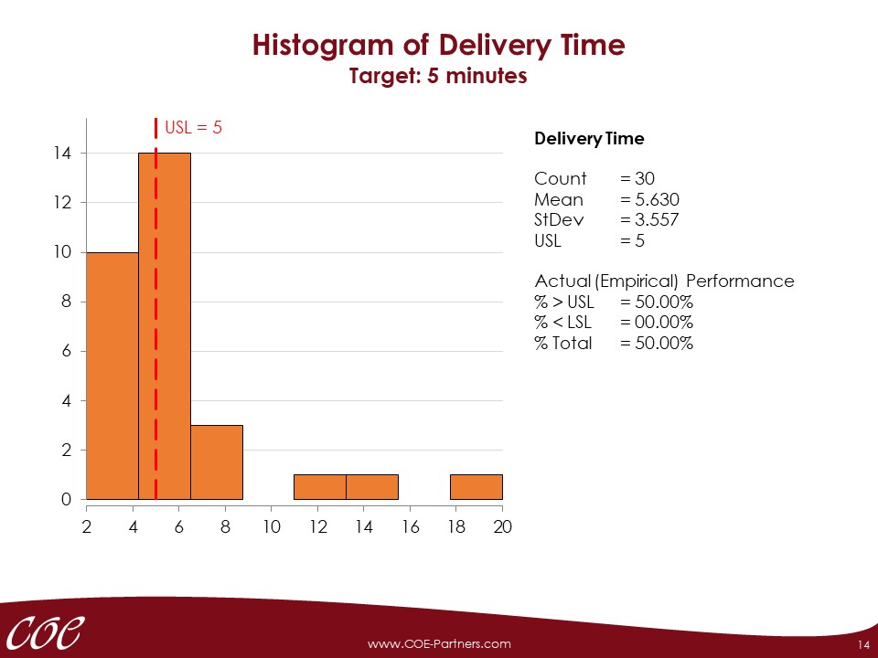
In addition to a time study, it is important to know the distribution of the data. It is very likely that continuous data in an undisturbed process, that means a process with only common cause variation, delivers a distribution similar to a normal one. In case the distribution is exceedingly different from a normal distribution, there could potentially be systematic influence factors, such as process changes. The graphical analysis of a distribution can be done using histograms, dotplots or boxplots. Additionally, a probability plot can be used to check the distribution of a sample for normality.
This step has the following deliverables:
- A series of graphical displays for collected data.
5. Calculate Process Capability
Apart from the graphic representation of the data collected, it is important to determine the current process results, since at the beginning of a project these can often only be estimated.
The purpose of this step is to calculate the actual process results, and if necessary, to correct the estimated value placed in the project charter. It is possible that this also results in adapting the project objective and/or scope.
Conclusion – Lean Six Sigma MEASURE Phase
After the Lean Six Sigma MEASURE phase has been completed by undergoing the above mentioned tasks, the Lean Six Sigma phase ANALYSE can be started.
This Lean Six Sigma Measure phase has the following deliverables:
- A fishbone diagram with clusters of potential root causes like machine, method, material, man and mother nature or project specific clusters that have become apparent during development of potential root causes,
- List of potential root causes that have been selected for data collection based on process knowledge and experience of the team members,
- List of measurement systems used for data collection,
- A data collection plan showing what measurements are to be taken by whom, when, where, how, under which conditions etc.,
- Matching data sets for problem and potential root causes,
- Graphical displays for collected data and
- Descriptive indicators for collected data.
Proceed to ANALYSE


